


1.完整项目描述和程序获取
>面包多安全交易平台:https://mbd.pub/o/bread/Y5qZmp9y
>如果链接失效,可以直接打开本站店铺搜索相关店铺:
>如果链接失效,程序调试报错或者项目合作也可以加微信或者QQ联系。
2.部分仿真图预览

3.算法概述
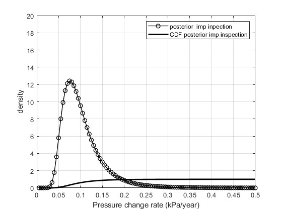
根据贝叶斯概率论可知,某一事件的后验概率可以根据先验概率来获得,因此,这里首先对事件的先验概率分布进行理论的推导。假设测量的腐蚀数据服从gamma分布,完备集下的后验概率不太适用于实际情况,因此,对于实际情况,需要考虑非完备集下的后验概率的计算。非完备集下的后验概率是关于随机事件的条件概率,是在相关证据给定并纳入考虑之后的条件概率。
4.部分源码
K_d = length(dt(:,:,kk1)); %total number of d
K_l = length(Lt(:,:,kk1)); %total number of l
for i = 1:K_d
if Nn2(i) == 1
dt1(i,:,kk1) = dt1(i,:,kk1);
else
dt1(i,:,kk1) = 5.39 + 0.19*dt1(i,:,kk1) - 0.02*Lt(i,:,kk1) + 0.35*Nn2(i);
end
end
%m->mm
dt1 = 1000*dt1;
%to obtaion a average number of do_rate and Lo_rate
do_rate = sum(dt1(:,:,kk1))/K_d;
Lo_rate = sum(Lt(:,:,kk1))/K_l;
% Q = sqrt(1+0.31*power(Lo_rate/sqrt(D/t),2));
% Q--length of correction factor
Q1 =(Lo_rate/sqrt(D_t))^2;
Q = sqrt(1+0.31*Q1);
% pf_rate=(2*t*sigma_u*(1-do_rate/t))/(D-t)/(1-(do_rate/t)/Q);
% pf -- failure pressure
pf_rate_1 = 2*t*sigma_u*(1-do_rate/t);
pf_rate_2 =(D-t)*(1-do_rate/t/Q);
pf_rate = pf_rate_1/pf_rate_2;
grid_dist = 0.1/20; % in order to get the obvious result on the plot
x = grid_dist:grid_dist:pf_rate*0.015;
%fit the contineous inverted gamma density to the data
par = invgamafit(0.1); % change pf_rate from mPa to kPa, in order to get the obvious result on the plot
a = par(1);
b = 1/par(2);
%Examining inverted gamma distributed prior
prior = exp(a*log(b)-gammaln(a)+(-a-1)*log(x)-b./x);
load r2.mat
prior = post_imp_prior';
%Examination of inverted gamma post prior after perfect inspection
A = a + dt1(K_d)/pf_rate^2;
B = b + Lt(K_l)/pf_rate^2;
postprior = exp(A*log(B)-gammaln(A)-(A+1)*log(x)-B./x);
%***********************************************************************************
% % %***********************************************************************************
% %定义likelyhood
% likeliprod = likelihoods(x,t,dt(:,:,kk1),Lt(:,:,kk1),Nn2);
%***********************************************************************************
%这个部分和之前的不一样了,修改后的如下所示:
%***********************************************************************************
%对prior参数进行随机化构造
m = 10;
for ijk = 1:m
ijk
%Calaulate the depth change rate and length change rate with time
for kk1 =1:(kk -1);
drate1 = normrnd(drate,drateS, nsamples,1, kk1); % Measured defect depth @ time T
Lrate1 = normrnd(Lrate,LrateS, nsamples,1, kk1); % Measured defect length @ time T
if kk1 == 1
dt(:,:,kk1) = do1(:,:,kk1) + drate1(:,:,kk1)*(delT) ;
dt1(:,:,kk1) = dt(:,:,kk1);
Lt(:,:,kk1) = Lo1(:,:,kk1) + Lrate1(:,:,kk1)*(delT) ;
else
dt(:,:,kk1) = dt(:,:,kk1-1) + drate1(:,:,kk1)*(delT);
dt1(:,:,kk1) = dt(:,:,kk1) ;
Lt(:,:,kk1) = Lt(:,:,kk1-1) + Lrate1(:,:,kk1)*(delT);
end
end
K_d = length(dt(:,:,kk1)); %total number of d
K_l = length(Lt(:,:,kk1)); %total number of l
for i = 1:K_d
if Nn2(i) == 1
dt1(i,:,kk1) = dt1(i,:,kk1);
else
dt1(i,:,kk1) = 5.39 + 0.19*dt1(i,:,kk1) - 0.02*Lt(i,:,kk1) + 0.35*Nn2(i);
end
end
%m->mm
dt1 = 1000*dt1;
%to obtaion a average number of do_rate and Lo_rate
do_rate = sum(dt1(:,:,kk1))/K_d;
Lo_rate = sum(Lt(:,:,kk1))/K_l;
% Q = sqrt(1+0.31*power(Lo_rate/sqrt(D/t),2));
% Q--length of correction factor
Q1 =(Lo_rate/sqrt(D_t))^2;
Q = sqrt(1+0.31*Q1);
% pf_rate=(2*t*sigma_u*(1-do_rate/t))/(D-t)/(1-(do_rate/t)/Q);
% pf -- failure pressure
pf_rate_1 = 2*t*sigma_u*(1-do_rate/t);
pf_rate_2 =(D-t)*(1-do_rate/t/Q);
pf_rate = pf_rate_1/pf_rate_2;
grid_dist = 0.1/20; % in order to get the obvious result on the plot
x = grid_dist:grid_dist:pf_rate*0.015;
%fit the contineous inverted gamma density to the data
par = invgamafit(0.1); % change pf_rate from mPa to kPa, in order to get the obvious result on the plot
as(1,ijk) = par(1);
bs(1,ijk) = 1/par(2);
%***********************************************************************************
%***********************************************************************************
end
npar = m; % dimension of the target
drscale = m; % DR shrink factor
adascale = 2.4/sqrt(npar); % scale for adaptation
nsimu = 5e5; % number of simulations
c = 10; % cond number of the target covariance
a = ones(npar,1); % 1. direction
[Sig,Lam]= covcond(c,a); % covariance and its inverse
mu = 1.35*as;% center point
model.ssfun = inline('(x-d.mu)*d.Lam*(x-d.mu)''','x','d');
params.par0 = mu+0.1; % initial value
params.bounds = (ones(npar,2)*diag([0,Inf]))';
data = struct('mu',mu,'Lam',Lam);
options.nsimu = nsimu;
options.adaptint = 100;
options.qcov = Sig.*2.4^2./npar;
options.drscale = drscale;
options.adascale = adascale; % default is 2.4/sqrt(npar) ;
options.printint = 100;
[Aresults,Achain]= dramrun(model,data,params,options);
mu = bs;% center point
model.ssfun = inline('(x-d.mu)*d.Lam*(x-d.mu)''','x','d');
params.par0 = mu+0.1; % initial value
params.bounds = (ones(npar,2)*diag([0,Inf]))';
data = struct('mu',mu,'Lam',Lam);
options.nsimu = nsimu;
options.adaptint = 100;
options.qcov = Sig.*2.4^2./npar;
options.drscale = drscale;
options.adascale = adascale; % default is 2.4/sqrt(npar) ;
options.printint = 100;
[Bresults,Bchain]= dramrun(model,data,params,options);
%选择值最集中的最为最终的值;
for i = 1:m
[Na,Xa] = hist(Achain(:,i));
[V,I] = max(Na);
A1(i) = Xa(I);
[V,I] = min(Na);
A2(i) = Xa(I);
[Nb,Xb] = hist(Bchain(:,i));
[V,I] = max(Nb);
B1(i) = Xb(I);
[V,I] = min(Nb);
B2(i) = Xb(I);
end
As = mean(A1);
Bs = mean(B1);
post_imp_prior = exp(As*log(Bs)-gammaln(As)-(As+1)*log(x)-Bs./x);
post_imp_prior_CDF = cumsum(post_imp_prior)*grid_dist;
A137